PostgreSQL JSONB vs MongoDB BSON: The Real Architectural Tradeoffs

Most teams pick between Postgres and Mongo by arguing about SQL vs documents, transactions, joins, or what everyone's using at the moment. The format on disk barely makes it into the discussion. That’s the wrong place to stop, because each database’s byte level design carries the philosophy of the engine. BSON is a binary echo of MongoDB's runtime: a self describing wire format that the server can scan, mutate, and ship easily. JSONB is a parse tree frozen into a Postgres tuple: optimized for read time access, indifferent to write time mutation, and beholden to MVCC.

Once you know what each format actually is, the rest of the comparison stops being a religious argument and starts being a set of engineering tradeoffs you can reason about. This piece walks through what BSON and JSONB are at the byte level, how they behave once they hit storage, what each one costs to index, update, and read back, and which workloads each one quietly punishes.

Why the format matters more than the API

Application developers see JSON. Both engines accept JSON on the way in and serve JSON on the way out, so it is tempting to assume the storage format is a cosmetic detail. It is not. The storage format dictates:

How much byte juggling the server does on every read.
Whether a partial update can mutate a value in place or has to rewrite the entire document.
What kinds of indexes can be built and how big they get.
How much write amplification you pay when a single field changes.
Whether the disk representation survives a torn page or a partial flush.

A query that runs in 1ms on a hot row can run in 30ms if the format forces the server to materialize and reparse the row. A field update that flips a boolean can rewrite 8KB of heap, generate WAL, trigger toast churn, and invalidate three indexes, or it can patch four bytes. The format decides which world you live in.

BSON: a binary echo of MongoDB's runtime

BSON stands for Binary JSON. BSON is a length prefixed, type tagged, ordered key value format that was designed with three properties in mind: cheap to parse linearly, cheap to mutate in place when the new value is the same size, and rich enough to carry types that JSON cannot express.

The wire layout of a BSON document looks roughly like this:

int32  total_document_length_in_bytes
{ element }*
byte   0x00  // terminator

Each element is itself:

byte    type_tag    (0x01 double, 0x02 string, 0x03 embedded doc, 0x07 ObjectId, ...)
cstring field_name
<payload depending on type>

Two things follow from that layout. First, every document and every embedded subdocument carries its own length prefix, which means a parser can skip an entire subtree in one pointer arithmetic step. Second, fields are ordered. The same logical document can be encoded in different byte sequences depending on insertion order, and the server preserves that order.

The type tag set is wider than JSON's. BSON has dedicated tags for:

32 bit and 64 bit integers (JSON has only a generic number).
IEEE 754 decimal128 for financial workloads.
ObjectId (12 bytes: timestamp, machine id, counter).
UTC datetime (int64 milliseconds since epoch).
Binary blobs with a subtype byte.
UUID (a binary subtype).
Regular expressions.
A JavaScript code type, mostly historical.
MinKey and MaxKey sentinels used for index bounds.

Two consequences for engineers. One: BSON round trips numeric types faithfully. A column that stores 64 bit account ids does not silently become a double the way it would in pure JSON. Two: BSON carries metadata that JSON cannot, which is part of the reason a MongoDB driver feels chatty when you push it through a strict JSON pipeline.

The clever bit, and the one that distinguishes BSON from a hundred other binary JSON formats: every field's payload is preceded by enough information that a server can walk the document linearly without recursive parsing, and many field updates can be performed by patching the payload in place. If you change an int32 field from 7 to 8, the document length does not change, the field offset does not move, and the engine writes four bytes. That property is what lets WiredTiger keep update latency flat across a wide range of document sizes.

It also explains the cost of BSON. Field names are stored as raw cstrings in every document. A collection of a billion documents with a created_at field carries the literal bytes created_at\0 a billion times. There is no schema, no dictionary, no shared symbol table. Wide documents with long field names waste a lot of disk and a lot of memory.

JSONB: a parse tree frozen on disk

JSONB is the spiritual opposite of BSON. Where BSON is a wire format that happens to live on disk, JSONB is a storage format that happens to be transferable. Postgres parses incoming JSON, normalizes it (keys sorted, whitespace stripped, duplicate keys deduplicated with last write wins), and serializes the result into a binary structure that maps directly onto the engine's value tree.

There is no public byte spec the way there is for BSON. Internally, a JSONB value is a header plus a sequence of entries that describe each key value pair, plus the data area. The headers contain length and type bits so the engine can binary search keys inside an object, and offsets are stored every N entries to bound the cost of finding a specific key. That structure has two big implications.

First, JSONB is a read optimized format. Once the document is stored, looking up a key by name is logarithmic in the number of keys, not linear. For wide objects with hundreds of fields, this matters. BSON, by contrast, is linear: it walks the document until it finds the key, leveraging the length prefixes to skip subtrees.

Second, JSONB cannot be patched in place. The header layout, the offset cache, and the dedup pass all assume the value is being constructed from scratch. Updating a single boolean inside a 4KB JSONB document materializes a brand new 4KB JSONB document, writes a new heap tuple, marks the old one dead, and updates every index that references it. This is not a JSONB design flaw, it is the consequence of binding the format to Postgres's MVCC and TOAST machinery. JSONB does what makes Postgres fast at reads. Postgres pays for the rest at write time.

JSONB throws away two things compared to JSON. Key order is lost (objects are stored with keys sorted), and duplicate keys are collapsed. Most applications never notice, but if you are relying on either property, you want json (the text type) not jsonb. Almost nobody should be relying on either property.

JSONB also does not preserve numeric type fidelity in the same way BSON does. Postgres has its own numeric type which is arbitrary precision, and JSONB encodes numbers using that representation. You will not lose precision the way you would with a 64 bit float, but you also do not get a distinct int32 vs int64 tag the way BSON gives you.

Binary blobs and where the type systems leak

The gap between BSON and JSONB shows up the fastest when data falls outside JSON's native type system.

Binary blobs are the usual offender. BSON has a native binary type with a subtype tag, JSONB does not. In Postgres your options are base64 encoding the bytes into JSONB (ugly), or pulling them out into a separate bytea column and referencing them by id (cleaner). Splitting the document works fine when you own the schema, it becomes awkward when you are ingesting third party documents that already embed binary fields, like S3 events with attachments or message payloads with thumbnails.

Storage: WiredTiger pages vs heap tuples plus TOAST

The byte format is half the story. The other half is what the storage engine does with the bytes.

MongoDB stores BSON documents inside WiredTiger, a B+ tree storage engine that also backs a number of other databases. WiredTiger gives MongoDB two important properties:

Block compression by default. Snappy compresses each block; zstd is available and can roughly halve the disk footprint on text heavy collections. The compression happens at the storage layer, so the in memory representation is uncompressed but the on disk and on wire (replication) footprint is much smaller. For a workload that stores web event payloads or product catalogs, the ratio of on disk size to logical size is routinely 3:1 or better.
In place updates when possible. If a field changes and the new BSON encoding fits in the existing slot, WiredTiger patches the page. If the document grows beyond its allocated space, WiredTiger rewrites the document, which is the expensive path. Schema decisions matter here: documents with arrays that grow over time will rewrite often, and the standard advice is to size arrays carefully or break them out into separate collections.

WiredTiger maintains a journal (write ahead log) that commits to disk every 100ms by default, and snapshots dirty pages to disk at 60 second checkpoints. The two intervals together keep recovery time bounded without grinding the write path on every commit.

PostgreSQL stores JSONB inside a heap tuple, the same structure that holds every other Postgres row. The heap is a page based store (8KB pages by default) with row level MVCC. Every update writes a new tuple, links it to the old one, and lets autovacuum reclaim the dead copy later.

JSONB also interacts with TOAST (The Oversized Attribute Storage Technique). Any column value that exceeds approximately 2KB after compression gets pushed into a separate TOAST table and replaced in the main heap with a pointer. JSONB documents larger than that threshold therefore live in two places: the heap tuple holds a pointer, and the actual JSONB lives in toast chunks. Reading the document means following the pointer and reassembling the chunks. The default TOAST strategy for jsonb is EXTENDED, which means values are first compressed (using the cluster's default compression, pglz or lz4 since PG 14), and then chunked if still over threshold.

The two consequences are easy to miss:

A SELECT * on a table with TOASTed JSONB columns will fetch the entire chain even if you only wanted three scalar fields from the row. Project the columns you need or extract the JSONB fields explicitly.
Updating one field in a JSONB document materializes a new JSONB, which gets TOASTed again. The old TOAST chunks become dead and wait for autovacuum. On a heavy update workload against large JSONB documents, the TOAST table can balloon faster than the main heap.

Postgres 14 added LZ4 compression for TOAST, which is meaningfully faster than the legacy pglz both for compression and decompression. If your JSONB columns are large and updated often, switching to LZ4 is the single highest leverage TOAST change you can make.

Updates: in place vs MVCC tombstones

Spend ten minutes profiling a heavy update workload on each engine and the contrast jumps out.

In MongoDB, a field level update with $set, $inc, or $push is interpreted by the server and translated into a targeted mutation of the BSON document. If the new value fits, WiredTiger updates the page in place. If it does not fit, the document is rewritten. Index entries are only touched for the fields that actually changed and that are indexed. The journal records the delta, not the whole document.

In PostgreSQL, UPDATE on a JSONB column always rewrites the entire JSONB value. The jsonb_set function looks surgical at the SQL layer (it lets you set a specific path) but underneath, it builds a new JSONB and the row update replaces the old tuple. MVCC then leaves a dead tuple behind, autovacuum reclaims it later, and every index on the table that does not satisfy the HOT (Heap Only Tuple) conditions has to insert a new entry pointing at the new tuple. If your indexes reference fields inside the JSONB column, HOT is off the table and every update is amplified.

In practice this means two patterns dominate.

MongoDB rewards documents with mutable internals. A counter inside a document, a status field that flips often, an array that gets pushed to on every event: these are cheap operations. The flip side is that document growth is the silent killer. A document that starts at 1KB and grows to 50KB over a year is rewritten by WiredTiger every time it crosses its current allocation, which means the late life updates are dramatically more expensive than the early life updates.

PostgreSQL rewards documents that are read more than they are updated. Catalog data, feature flags, event payloads that are written once and read many times, configuration that changes weekly rather than per second: JSONB is excellent for these. The moment you start treating a JSONB document as a per row mutable object that changes on every request, you are fighting the engine.

The benchmark that exposes this gap is straightforward. Take a million row table or collection, each row holding a 4KB document with a view_count integer somewhere inside it. Increment the counter once per second per row across all rows. MongoDB may only need to modify the bytes associated with the changed field, avoiding the full document rewrite that JSONB incurs. Postgres rewrites 4KB of JSONB per document, generates 4KB of WAL per update, and starts producing dead tuples faster than autovacuum can clean them. The Postgres answer here is simple: do not store view_count in JSONB. Pull it into a regular bigint column. That fix is real and lasting, and it is also a tax on schemas that try to be JSON first.

Indexes: GIN, multikey, and what each can answer

Both engines let you index inside documents. The mechanisms are different, and the resulting indexes have different shapes.

PostgreSQL offers two index strategies for JSONB.

GIN indexes on the whole document. The default operator class supports containment (@>), key existence, and path queries. A more aggressive variant, jsonb_path_ops, supports only @> but produces a smaller, faster index. Both are inverted indexes that emit one entry per path through the document.

CREATE INDEX idx_events_data ON events USING GIN (data jsonb_path_ops);
SELECT * FROM events WHERE data @> '{"type": "signup"}';

B tree indexes on specific expressions. When you know the exact path you want to query, an expression B tree is dramatically smaller and faster.

CREATE INDEX idx_events_user_id ON events ((data->>'user_id'));
SELECT * FROM events WHERE data->>'user_id' = '12345';

MongoDB indexes work on field paths directly. The standard createIndex({user_id: 1, created_at: -1}) builds a B tree on a compound path. The syntax is different from Postgres, but the behavior is familiar.

Multikey indexes. When the indexed field is an array, MongoDB automatically creates one index entry per array element. The same B tree, traversed differently. A document with tags: ["postgres", "mongodb", "bson"] generates three index entries pointing at the same document, and any element match query can use the index. This is the killer feature for tags, references, and other array shaped data.

For fixed, known query shapes, Postgres ties or beats Mongo with expression B trees. For varied or array heavy data, Mongo's first class multikey support gives it more leverage with less ceremony.

One more thing Postgres has on Mongo here: partial indexes with arbitrary predicates. You can build an index that only covers the rows where some JSONB field has a specific value, or a date range, or whatever. Mongo has partial indexes too but the filter expressions you can use are way more limited, so anything more than a simple equality check usually has to live in the query side instead of the index.

Read paths and the cost of materialization

The end to end read path is where the two formats earn or lose their reputation.

A MongoDB find that hits an index and returns a single document does roughly the following: traverse the B tree to find the record id, fetch the page from WiredTiger, decompress the block, locate the BSON document inside the page, copy it into the response buffer, ship it over the wire. The document is already in BSON. If the driver supports it (most do), the bytes can travel from the storage page to the client with no parse on the server side. Field projection ($project in aggregation, or projection on find) walks the BSON in place and emits a trimmed version.

A PostgreSQL select that hits an index and returns a single row does roughly the following: traverse the B tree to find the heap tuple location, check the visibility map and the tuple's xmin/xmax to confirm the row is visible to this transaction, fetch the heap page, locate the tuple, follow any TOAST pointers to reassemble JSONB columns, materialize the row into the executor's tuple format, apply any projections, and emit. The visibility check is the MVCC tax. The TOAST chase is the wide column tax. The materialization is the format tax.

For point reads of small documents, both engines are fast and the differences are noise. For wide documents (tens of KB) or selective projections on a large document, BSON has a structural edge because the on disk format and the on wire format are the same, and projection is a walk. JSONB has to be unpacked and the projection produces new JSONB. The win is not huge in absolute terms, but it shows up on workloads that fan out reads.

Aggregations flip it though. Postgres has been working on its query planner for like 30 years. Parallel scans, hash joins, merge joins, a cost based optimizer that has seen basically every shape of analytical query a person can write. Mongo's aggregation pipeline has gotten way better in recent versions (SBE is faster, $lookup is actually usable now), but once you're doing real analytics with multiple joins and big group by aggregates, Postgres just wins. Not by a small margin either, you'll often see big multiples on the same workload.

When PostgreSQL JSONB is the right answer

Reach for JSONB when:

The bulk of your schema is relational and a few columns happen to be semi structured. Customer records with a metadata field. Products with a variable attributes blob. Orders with line items that have inconsistent shape across categories.
Reads dominate writes against the JSONB columns. Catalog data, configuration, audit payloads, settings.
You need joins. Postgres can join JSONB columns against regular columns against full text indexes against PostGIS geometries against time series partitions in one query. Mongo can do this through $lookup but it is not the same.
You need transactions across many rows. JSONB inherits Postgres's transaction model for free.
The team is already running Postgres and the operational cost of adding a second database is not justified.
You want strong typing in some columns and document flexibility in others, in the same table.

Workloads that fit this shape: SaaS application data, e commerce catalogs, CMS storage, configuration stores, audit logs that need to be queried by structured fields, anything where the analytical query layer is going to use SQL anyway.

When MongoDB BSON is the right answer

Reach for MongoDB when:

The unit of work is the document. Each request reads or writes one document, occasionally a few. Most operations do not span documents.
Documents are large, mutate frequently, and the mutations are field local. Telemetry events that get enriched over time. Game state. IoT device shadows. Anything where the same document gets touched many times and each touch is small.
The query patterns are varied and the schema is genuinely fluid. You do not know which fields users will query next month.
You need horizontal write scaling out of the box. Mongo's native sharding has gotten very good. Postgres has sharding solutions (Citus, partitioning) but they are bolted on rather than first class.
You need a document oriented secondary index pattern that Postgres expression indexes cannot model cleanly.
The team has Mongo expertise and the workload does not need SQL analytics.

Workloads that fit this shape: real time event streams with rich payloads, mobile and game backends, IoT device fleets, content management with deeply nested structures, anything where the data model is naturally a graph of nested objects and the queries are mostly key value style with occasional secondary lookups.

The practical takeaway

If you remember three things from this:

The format is the engine. BSON is what makes Mongo fast at field updates and fast at projection. JSONB is what makes Postgres flexible without giving up relational performance. The choice between them is not about JSON vs binary, it is about update behavior, index shape, and read path.
JSONB is a read optimized format. It pays for itself when you write once and read many. It punishes you when you treat a JSONB column as a mutable object that changes on every request. Pull hot mutable fields out into regular columns.
BSON is an update optimized format. It pays for itself when documents are touched often and the touches are local. It punishes you when documents grow unboundedly, when field names are long, and when the query pattern wants joins and aggregations.

Pick the engine whose architectural assumptions match your workload's access pattern. Everything else is a tax you will pay every day until you fix it.

Working with MongoDB documents?

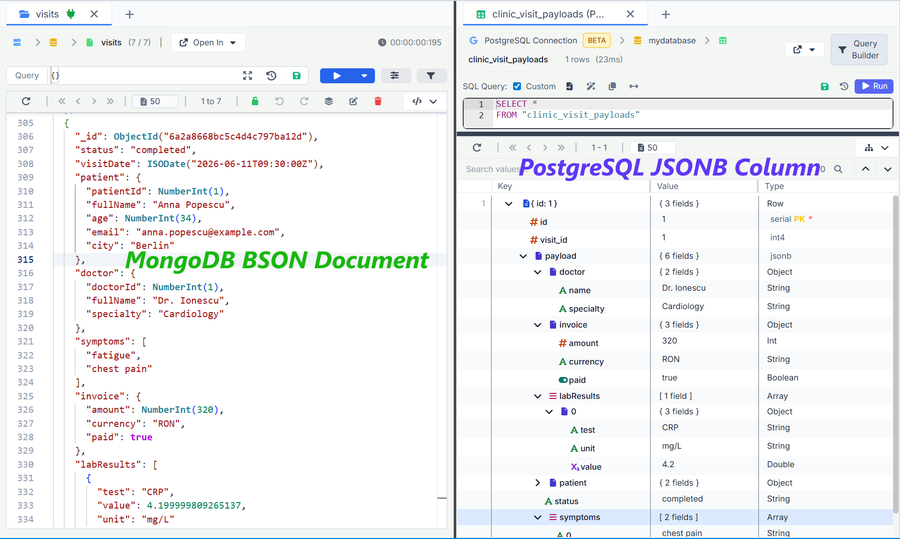
Understanding BSON is useful, but seeing the structure of your collections makes the work much easier.

With VisuaLeaf, you can browse MongoDB documents, inspect schemas visually, build queries, create aggregation pipelines, and understand how your data is actually organized.

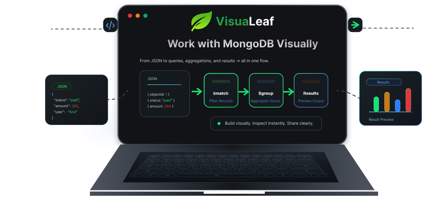
Try VisuaLeaf!

Download for Free